
Constant magnetic force separation systems generate the same conditions for all magnetic beads in the suspension. As bead behavior is consistent at every point of the working volume, any changes in the suspension's opacity can be directly related to changes in the suspension’s characteristics.
The biomagnetic separation curves, obtained by monitoring the opacity changes over time, allows users to characterize each product. For example, they can be used for comparing different batches of the same product (both curves should be the same). They can also be used to check the effect of the suspension variation in the magnetophoretic behavior. Aggregation would speed up the separation, increased viscosity would slow it, and higher concentration would reduce the separation time.
Under constant magnetic force conditions, a typical biomagnetic separation curve can be fitted with a sigmoidal function. The behaviour can then be described with four parameters:
- Opacity at the starting time (when t=0)
- Final opacity (at t=infinite)
- The slope (defined by the dimensionless exponent ‘p’)
- The half-separation time (t50, expressed in seconds)
Because the starting opacity increases with concentration, the opacity values provide information about the optical properties. This can vary due to sensitivity to small changes in the vessel's position: large volume systems need to have a large clearance to avoid accidents, especially when using glass vessels.
However, the information related to the magnetic separation (i.e., separation speed or magnetophoretic behavior) is contained in the t50 and p parameters. That is why, when comparing different samples, the opacity is usually normalized (initial opacity - final opacity = 100%).
A common problem users have when establishing an SOP for magnetic separation is determining the separation time. Identifying when the process has finished can be difficult, because the slope for t>>t50 is fairly flat. This means that any small variation in the criteria can lead to very different times. Even a small amount of noise in the optical measure can make it complicated to identify a threshold where the separation is complete.
However, if the sigmoidal fitting is good enough (let’s say, when its determination coefficient r2 >0.99), the values of t50 and p are very robust. It is easy to extrapolate the fitted parameters to t99, which is the value when the opacity has decreased by 99% of the difference between starting and final values. Note that the fitting also obtains the final opacity without the need to reach t=infinite.
For most biomagnetic separation process, a good criterion is to establish the separation time as tsep=t99 (when the slope ‘p’ is below 2, some users prefer to use 2*t99 or 3*t99). The value of t99 doesn’t needs to be determined from the final part of the curve but can be calculated directly from the t50 and p as t99=t50*99(1/p). In this example, the biomagnetic separation curve’s sigmoidal fitting gives the values of t50=57s and p=4.8. The separation time, defined as t99, would be 150s.
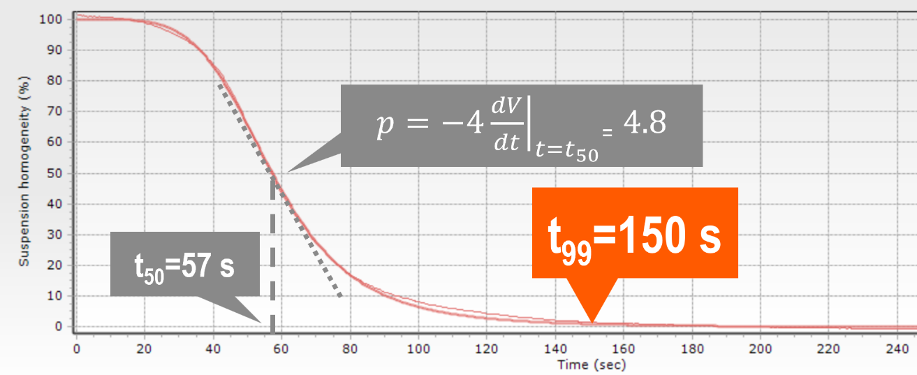
Figure 8.1 Graph showing the change in suspension homogeneity over time. t50 and p values are obtained by fitting the experimental data to a sigmoidal curve, then t99 is calculate as t99=t50*99(1/p)
Monitoring the biomagnetic separation process is not just a quality control tool for comparing the consistency of different batches. It is also a powerful tool to establish proper SOPs, allowing users to objectively set up the correct separation time for each product and process.
The old saying ‘magnetic beads don’t work at large volumes’ is, simply, wrong. If you want to learn what leading IVD-manufacturers already know, this is the e-book for you!

Related news
- Different types of Immunoassays
- DBCO click chemistry: what is it and what are its benefits?
- What is poly dt?