
Under constant magnetic force conditions, optical monitoring of the biomagnetic separation process provides information on both when the separation is complete and the characteristics of the magnetic bead suspension.
The absorbance/opacity time-change during separation can usually be fitted to a sigmoidal curve. The magnetophoretic behaviour can then be characterized by t50 (time when it reaches 50% of the difference between maximal and minimal absorbance) and the exponent ‘p’ (related to the slope of the curve at t50). These two values are quite robust, even when the experimental curve is not a perfect sigmoidal, but for simplicity we will limit the discussion to the cases when the determination coefficient, r2, is larger than 0.99.
Initially, fitting absorbance curves was used for quality control. For batches of the same product, the separation process should produce the same curve. In this context, if the values of t50 and p vary from those expected, then users could assume that something was wrong with the bead suspension.
Subsequently, using QCR software (an early version of the current Qualitance), we noticed that batches in Production Process usually deviated by a reduction of t50 and an increase of p. This demonstrated that when the magnetic beads are clumped, the separation is faster. Using this knowledge, production managers could identify the batches where the suspension was not properly processed, or the magnetic beads had not been stored correctly.
As a result, the R&D version of this tool (Monitor software) was used to test re-suspension protocols. When preparing the SOP, the protocol was tested by measuring the suspensions of the same batch after being stored and re-suspended according to the preliminary procedures.
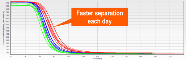
Figure 9.1 Graph showing the change in suspension homogeneity over time, where separation time declines over three days: day 1 (red), day 2 (blue) and day 3 (green). The suspension was measured several times on each day.
Figure 9.1, shows the separation time of a suspension, sampled on three separate days. On Day 1 (red), the suspension was measured several times, resuspending it between each measurement. The suspension was stored, and then measured again on Day 2 (blue). This was repeated for a third time on Day 3 (green). As you can see in Figure 9.1, the absorbance curve shows a faster separation time each day, which can be quantified by the decrease in t50 and the increase of p (Fig. 9.2).
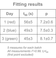
Figure 9.2 Table of results showing parameters t50 (s) and p and their errors on Days 1, 2 and 3.
Because the expected difference between the results on different days should be smaller than the error for both fitting parameters, t50 and p, these results should lead to a revision of their storage and re-suspensions protocols. Figure 9.3 shows the separation time where a 1 L bottle with the suspension stored on a roller was used, demonstrating improved reproducibility of the magnetic separation curve.
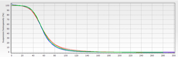
Figure 9.3 Graph showing the change in suspension homogeneity over time, where a 1 L vessel with the suspension stored on a roller was used, demonstrating improved reproducibility of the magnetic separation curve.

Figure 9.4 Table of results for the graph in Fig.9.3, showing parameters t50 (s) and p and their errors.
With a confidence interval of >95%, the data from the first 20 batches can be used to define the t50 and p, and their errors (defined as 2σ). If the distribution of the errors is normal and the process is reproducible, no more than one curve should show its fitting parameters (t50 and p) outside of the error margins. That is, only one in 20 measures can have t50 and/or p values below <t50>-2 σt50 or over <t50>+2 σt50 (and the same for p).
Users should keep in mind that even if the magnetic force is constant, the separation speed (and therefore the separation time) is the result of the competition between the magnetic force and the drag force. Because drag force depends on the viscosity of the suspension, it is important to remember that the suspension’s viscosity will vary with temperature. From 18 ºC to 24 ºC the viscosity changes by 15% (5% from 20 to 22ºC) which is reflected in a similar decrease of t50.
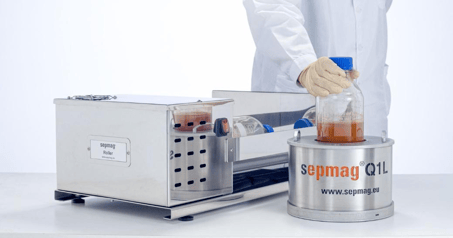
Figure 9.5 Advanced Biomagnetic Separation system Sepmag Q1 L equipment and re-suspension equipment Sepmag Roller.
When using constant magnetic force systems, quantifying and parametrizing absorbance changes during separation are a powerful tool for quality control. They are also key to investigating how different steps may affect the suspension, helping to establish robust SOPs.
The old saying ‘magnetic beads don’t work at large volumes’ is, simply, wrong. If you want to learn what leading IVD-manufacturers already know, this is the e-book for you!

Related news
- Different types of Immunoassays
- DBCO click chemistry: what is it and what are its benefits?
- What is poly dt?